Create an Alpha Model based strategy#
A different approach to strategies implementation involves the use of Alpha Models. The backtesting module contains both an abstract AlphaModel and an AlphaModelStrategy - a base strategy, which puts together models and all settings around it.
Note
Review How to backtest your strategy first - especially the Prerequisites section
(DummyTicker, demo_data_provider, and get_demo_settings()). The alpha-model tutorial
uses the same demo setup so you can run examples without downloading the entire demo_scripts folder.
Alpha Model vs Abstract Strategy#
Both approaches run inside the same event-driven backtester, but they split work differently.
Abstract Strategy (see How to backtest your strategy) is the lower-level option. You subclass
AbstractStrategy and implement calculate_and_place_orders(). In that method you typically:
fetch prices from
ts.data_provider,decide what to do,
build orders with
OrderFactory,send them to the
Broker.
You control the full pipeline. That flexibility is useful when order logic is unusual (for example, custom sizing, staged entries, or logic that does not map cleanly to a single directional view per asset). It also means more code and more moving parts on your side.
Alpha Model is the higher-level, more plug-and-play option. You subclass AlphaModel and
implement only calculate_exposure() - a directional view per ticker (LONG, SHORT, or OUT).
AlphaModelStrategy wires your models to the session, turns exposures into Signals, and lets a
PositionSizer convert those signals into concrete orders. You do not call the broker or order
factory yourself unless you extend the framework.
In short:
Abstract Strategy |
Alpha Model |
|
|---|---|---|
What you implement |
Full |
|
Who places orders |
You, via |
|
Level of control |
Boilerplate, more control |
Plug-and-play, focus on the signal, sizing is delegated |
When to choose |
You need custom execution or non-standard order flow |
You want reusable signal logic and standardised portfolio sizing |
Neither approach is “more advanced” in the sense of being harder to learn - they target different levels of abstraction. You might prefer to use Alpha Models for research and prototyping, and drop down to an Abstract Strategy when production execution rules do not fit the alpha-model pipeline.
Understanding Exposure#
An Exposure is the directional view your alpha model returns for one asset at one point in time.
QF-Lib represents it with the Exposure enum:
Exposure.LONG- you want a long position (buy and hold the asset, or increase an existing long).Exposure.SHORT- you want a short position (profit when the price falls).Exposure.OUT- you want to be flat (no position in that asset).
In the moving-average example below, the model only answers “should we be long or short?” It does not specify how many shares or what notional to trade. That is intentional: the alpha model expresses what to do and the PositionSizer decides how much to trade.
For example, the default SimplePositionSizer invests 100% of portfolio value in each signal
(fully long or fully short per asset, depending on configuration). Other sizers use a fixed percentage
of the portfolio or risk-based sizing from signal metadata (fraction_at_risk, and similar fields).
So returning Exposure.LONG is enough because you separate direction from size. If you need
both in one place, use an Abstract Strategy and call
OrderFactory.target_percent_orders() (or another helper) with explicit percentages yourself.
Simple Moving Average Alpha Model#
Let’s write our first Alpha Model strategy. The strategy will apply two Exponential Moving Averages of different time periods on the recent market close prices of the traded asset to determine the suggested move. It should suggest to go LONG on this asset if the shorter close prices moving average exceeds the longer one. Otherwise it should suggest to go SHORT. The code of the alpha model is available in the demo scripts.
At first we need to create the code of the new Alpha Model class. In order to use the AlphaModelStrategy it is necessary to
implement the AlphaModel.calculate_exposure() function, which returns the expected Exposure
for the given ticker (see Understanding Exposure above).
from qf_lib.backtesting.alpha_model.alpha_model import AlphaModel
from qf_lib.backtesting.alpha_model.exposure_enum import Exposure
from qf_lib.common.enums.price_field import PriceField
from qf_lib.common.tickers.tickers import Ticker
from qf_lib.data_providers.data_provider import DataProvider

class MovingAverageAlphaModel(AlphaModel):
    def __init__(self, fast_time_period: int, slow_time_period: int,
                 risk_estimation_factor: float, data_provider: DataProvider):
        super().__init__(risk_estimation_factor, data_provider)

        self.fast_time_period = fast_time_period
        self.slow_time_period = slow_time_period

    def calculate_exposure(self, ticker: Ticker, current_exposure: Exposure) -> Exposure:
        num_of_bars_needed = self.slow_time_period
        close_tms = self.data_provider.historical_price(ticker, PriceField.Close, num_of_bars_needed)

        fast_ma = close_tms.ewm(span=self.fast_time_period, adjust=False).mean()
        slow_ma = close_tms.ewm(span=self.slow_time_period, adjust=False).mean()

        if fast_ma[-1] > slow_ma[-1]:
            return Exposure.LONG
        else:
            return Exposure.SHORT
Let’s slowly review the implementation of the calculate_exposure function. At the very beginning we download the
historical prices from our data provider. To achieve this we use the historical_price function of the
DataProvider (injected into the model as self.data_provider). This function will return a pandas-compatible QFSeries.
Afterwards we apply the ewm() and mean() pandas functions to compute the fast and slow moving average. Finally, we return either Exposure.LONG when the fast moving average > slow moving average and Exposure.SHORT otherwise.
Some of the parts still may be confusing (what is the risk_estimation_factor?), but everything will be explained in later steps. Now let’s focus on running the alpha model to see the result of the strategy.
Run Alpha Model Strategy#
In order to run the strategy with the Alpha Model we just created we will need to use both BacktestTradingSession and AlphaModelStrategy.
AlphaModelStrategy is a predefined strategy which puts together alpha models and all settings around it and generates necessary orders. Let’s create a script to run the strategy at 1:00 a.m. every day.
import matplotlib.pyplot as plt
plt.ion()  # required for dynamic chart

from demo_scripts.common.utils.dummy_ticker import DummyTicker
from demo_scripts.demo_configuration.demo_data_provider import daily_data_provider
from demo_scripts.backtester.moving_average_alpha_model import MovingAverageAlphaModel
from demo_scripts.demo_configuration.demo_settings import get_demo_settings
from qf_lib.documents_utils.document_exporting.pdf_exporter import PDFExporter
from qf_lib.documents_utils.excel.excel_exporter import ExcelExporter

from qf_lib.backtesting.strategies.alpha_model_strategy import AlphaModelStrategy
from qf_lib.backtesting.trading_session.backtest_trading_session_builder import BacktestTradingSessionBuilder
from qf_lib.common.enums.frequency import Frequency
from qf_lib.common.utils.dateutils.string_to_date import str_to_date


def main():
    start_date = str_to_date("2010-01-01")
    end_date = str_to_date("2015-03-01")

    settings = get_demo_settings()
    pdf_exporter = PDFExporter(settings)
    excel_exporter = ExcelExporter(settings)

    session_builder = BacktestTradingSessionBuilder(settings, pdf_exporter, excel_exporter)
    session_builder.set_frequency(Frequency.DAILY)
    session_builder.set_data_provider(daily_data_provider)

    ts = session_builder.build(start_date, end_date)

    model = MovingAverageAlphaModel(fast_time_period=5, slow_time_period=20,
                                    risk_estimation_factor=1.25,
                                    data_provider=ts.data_provider)
    model_tickers = [DummyTicker('AAA')]
    model_tickers_dict = {model: model_tickers}

    strategy = AlphaModelStrategy(ts, model_tickers_dict)

    CalculateAndPlaceOrdersRegularEvent.set_daily_default_trigger_time()
    CalculateAndPlaceOrdersRegularEvent.exclude_weekends()
    strategy.subscribe(CalculateAndPlaceOrdersRegularEvent)

    ts.start_trading()


if __name__ == "__main__":
    main()
That’s it! Now you can run the script and monitor how well the strategy performs!
How does it actually work?#
When CalculateAndPlaceOrdersRegularEvent fires, AlphaModelStrategy.calculate_and_place_orders() runs.
The pipeline below is handled for you; your alpha model only participates in the first step.
Pipeline:
AlphaModel.calculate_exposure  →  Signal  →  PositionSizer.size_signals
     →  market orders (+ optional stops)  →  Broker.place_orders
Step by step
Signals - For each ticker,
AlphaModel.get_signal()calls yourcalculate_exposure()and wraps the result in aSignal(suggested_exposure,fraction_at_risk,last_available_price, and optional metadata). Signals are stored in the SignalsRegister for later analysis.Sizing -
PositionSizermaps each signal to a target portfolio percentage (or target value) and callsOrderFactory.target_percent_orders()(ortarget_value_orders()).Risk controls - If
use_stop_losses=True(default onAlphaModelStrategy), the sizer also createsStopOrderobjects fromfraction_at_riskandlast_available_price.Execution - Orders pass through any configured order filters, then the broker simulates fills.
The demo above uses the session default: SimplePositionSizer.
Pick another sizer on the builder before build():
session_builder.set_position_sizer(FixedPortfolioPercentagePositionSizer, fixed_percentage=0.2)
session_builder.set_position_sizer(InitialRiskPositionSizer, initial_risk=0.05)
session_builder.set_position_sizer(InitialRiskWithVolumePositionSizer, initial_risk=0.05, max_volume_percentage=0.1)
Built-in position sizers#
Class |
Role |
|---|---|
Default. Target weight = |
|
Scales each signal by |
|
Risk-based sizing: |
|
Same risk formula as |
See the backtesting API reference (position_sizer section) for parameters and sizing examples in each class docstring.
Final thoughts#
Alpha model can be a powerful tool to help you test your ideas and strategies. The backtest results usually provide a full picture of what happened every day, what was the performance of the strategy etc. In case if you would need to understand better why at certain point in time you were either LONG or SHORT, you could use a tool to plot your signals on top of a candle stick chart:
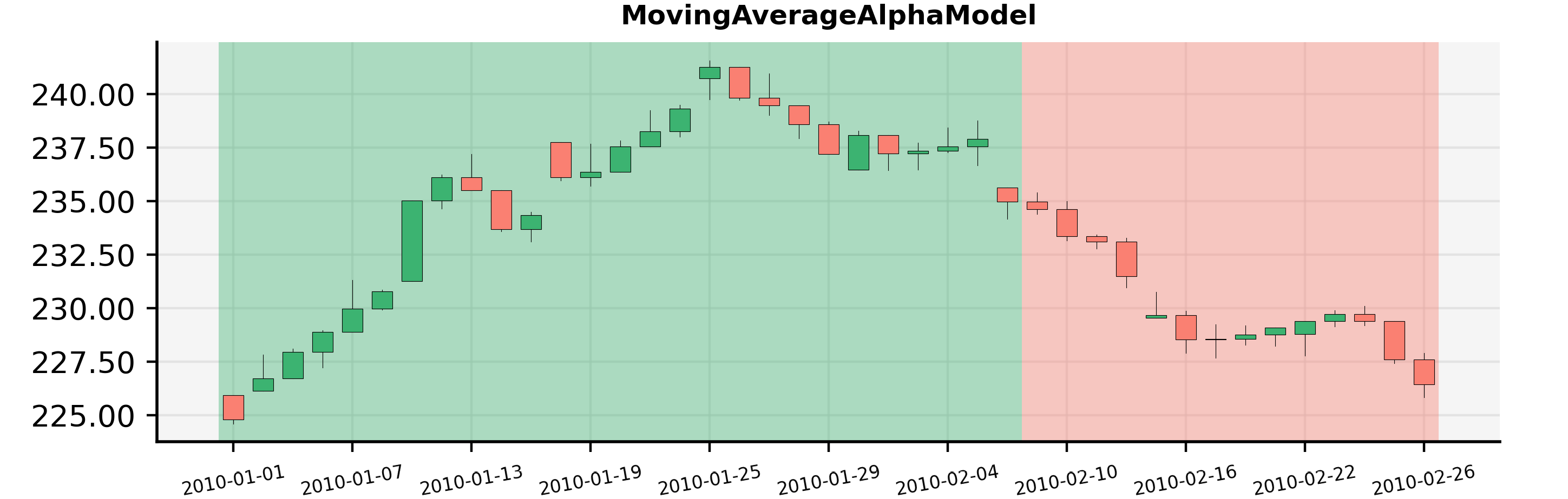
You can see here that the model was LONG for the given asset the whole January and became short around the 8th of February. To create the document with the chart you can use the following code sample:
from demo_scripts.backtester.moving_average_alpha_model import MovingAverageAlphaModel
from demo_scripts.common.utils.dummy_ticker import DummyTicker
from demo_scripts.demo_configuration.demo_data_provider import daily_data_provider
from demo_scripts.demo_configuration.demo_settings import get_demo_settings
from qf_lib.documents_utils.document_exporting.pdf_exporter import PDFExporter
from qf_lib.analysis.signals_analysis.signals_plotter import SignalsPlotter
from qf_lib.backtesting.events.time_event.regular_time_event.market_close_event import MarketCloseEvent
from qf_lib.backtesting.events.time_event.regular_time_event.market_open_event import MarketOpenEvent
from qf_lib.common.enums.frequency import Frequency
from qf_lib.common.utils.dateutils.string_to_date import str_to_date
from qf_lib.common.utils.dateutils.timer import SettableTimer
from qf_lib.documents_utils.document_exporting.pdf_exporter import PDFExporter
from qf_lib.settings import Settings


def main():
    start_date = str_to_date("2010-01-01")
    end_date = str_to_date("2010-03-01")
    signal_frequency = Frequency.DAILY
    title = "Signals Plotter Demo"

    # set market open and close time. Does not matter much for a backtest
    # signals will be calculated at midnight for daily frequency
    MarketOpenEvent.set_trigger_time({"hour": 8, "minute": 30, "second": 0, "microsecond": 0})
    MarketCloseEvent.set_trigger_time({"hour": 13, "minute": 0, "second": 0, "microsecond": 0})

    daily_data_provider.set_timer(SettableTimer(start_date))

    model = MovingAverageAlphaModel(fast_time_period=5, slow_time_period=20,
                                    risk_estimation_factor=1.25,
                                    data_provider=daily_data_provider)
    settings = get_demo_settings()
    pdf_exporter = PDFExporter(settings)

    plotter = SignalsPlotter([DummyTicker("AAA")], start_date, end_date, daily_data_provider,
                             model, settings, pdf_exporter, title, signal_frequency, data_frequency=signal_frequency)
    plotter.build_document()
    plotter.save()